
Are you tired of sifting through mountains of data in Excel, only to realize that you’ve been working with a bunch of duplicates?
Well, you’re not alone! Identifying and getting rid of duplicates in Excel is a common problem faced by many of us, but it’s also an important one.
Not only does it help to keep your data organized and accurate, but it also saves time and prevents errors in analysis.
In this blog post, we’ll go over the different methods for identifying duplicates in Excel, including some tips and tricks for troubleshooting along the way.
So whether you’re a seasoned Excel pro or just getting started, let’s dive in and learn how to tackle those pesky duplicates once and for all!
Methods for Identifying Duplicates
Okay, now that we understand the importance of identifying duplicates in Excel, let’s talk about the different methods we can use to do so.
Lucky for us, Excel offers several built-in tools that make the process easy and straightforward.
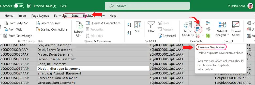
First up, we have the “Remove Duplicates” feature, which is located in the Data tab. This feature allows you to quickly and easily remove any duplicate rows from your data.
Simply select the range of cells that you want to check for duplicates, then click on the “Remove Duplicates” button.
Excel will then prompt you to select the columns that you want to check for duplicates, and voila! All of your duplicate rows will be removed.
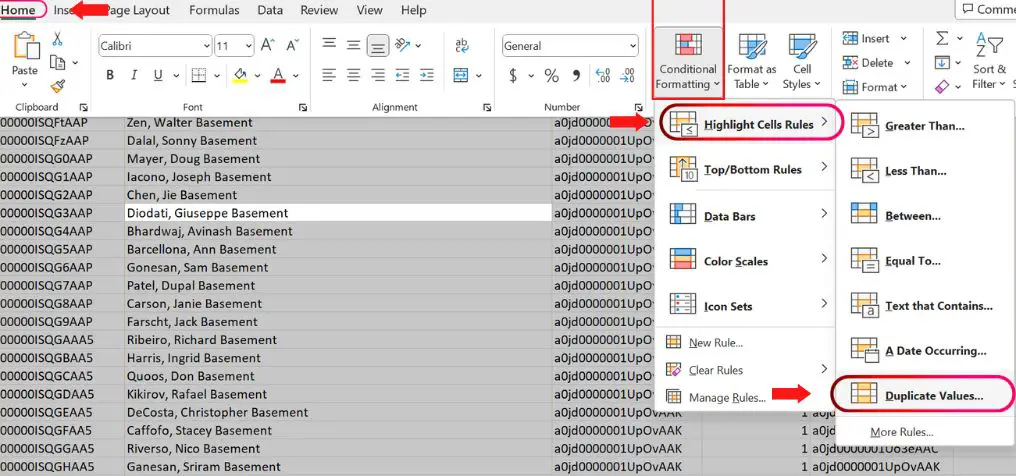
Next, we have the “Conditional Formatting” feature, which allows you to highlight any duplicate values in your data. This can be a great way to quickly spot any duplicates and make sure that they’re not causing any issues.
To use this feature, simply select the range of cells that you want to check for duplicates, then click on the “Conditional Formatting” button in the Home tab.
From there, you can select “Highlight Cells Rules” and then “Duplicate Values” to apply formatting to any duplicate values in your data.
Finally, we have the option to use a formula, such as COUNTIF or VLOOKUP, to identify duplicates. Both of these formulas allow you to compare data within your spreadsheet and identify any duplicate values.
COUNTIF, for example, returns the number of cells that meet a specified condition and VLOOKUP allows you to retrieve the value of a specific cell in the table.
This method requires a bit more knowledge of Excel’s functions and formulas, but it can be a powerful way to check for duplicates and even more advanced data manipulation.
So there you have it! Three simple yet effective ways to identify duplicates in Excel. You can choose the one that best suits your needs and start organizing your data like a pro!
Remove Duplicates Feature
All right, now that we’ve covered the different methods for identifying duplicates in Excel, let’s take a closer look at how to use the “Remove Duplicates” feature.
This is a great option if you want to quickly and easily get rid of any duplicate rows in your data, without having to manually scan through and delete them yourself.
And don’t worry, using this feature is simple and straightforward! Here’s a step-by-step guide to get you started:
Step 1: Select the range of cells that you want to check for duplicates. Make sure to include any headers or labels in your selection as well.
Step 2: Click on the “Data” tab, and then click on the “Remove Duplicates” button. You’ll see a pop-up window that lists all of the columns in your selected range.
Step 3: Select the columns that you want to check for duplicates. If you’re not sure which columns to select, you can just leave them all checked.
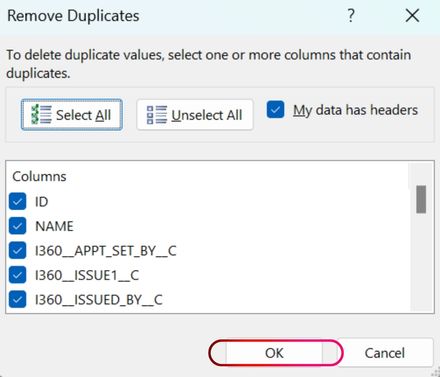
Step 4: Click on “OK” and Excel will then scan your selected range for any duplicate rows and remove them for you. A message will pop up that tell you how many duplicate values have been removed.
And that’s it! You’ve just used the “Remove Duplicates” feature to get rid of any duplicate rows in your data. Keep in mind that this feature will only remove exact duplicates and will not consider similar data.
Now, you can breathe a sigh of relief knowing that your data is clean and organized, and you can move on to your analysis with confidence!
Highlighting Duplicates with “Conditional Formatting” in Excel
Now that we’ve learned how to use the “Remove Duplicates” feature to get rid of any duplicate rows in our data, let’s take a look at how to use “Conditional Formatting” to highlight any duplicate values.
This is a great option if you want to quickly spot any duplicates and make sure that they’re not causing any issues. Plus, it’s a fun and colorful way to organize your data. Follow these simple steps to get started:
Step 1: Select the range of cells that you want to check for duplicates. Make sure to include any headers or labels in your selection as well.
Step 2: Click on the “Home” tab and then click on the “Conditional Formatting” button. From there, you can select “Highlight Cells Rules” and then “Duplicate Values”.
Step 3: When prompted, select the range of cells that you want to check for duplicates. Excel will then automatically apply formatting to any duplicate values in that range.
Step 4: You can choose the formatting you prefer, such as background color, font color or icon set.
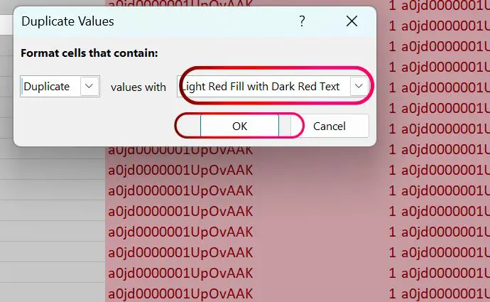
Step 5: Once you’re happy with the formatting, you can close the “Conditional Formatting” window.
And that’s it! You’ve just used “Conditional Formatting” to highlight any duplicate values in your data. It’s a quick and easy way to spot any duplicates and make sure that they’re not causing any issues.
It also makes it easier to read and scan large data sets. Now you’re ready to take your data analysis to the next level!
Using Formulas to Identify Duplicates in Excel (COUNTIF and VLOOKUP)
All right, now that we’ve gone over the “Remove Duplicates” feature and “Conditional Formatting” options, let’s dive into using formulas to identify duplicates in Excel.
This is a great option if you want more control over the process and are comfortable working with formulas. COUNTIF and VLOOKUP are two popular formulas that can be used for this purpose.
Both of these formulas allow you to compare data within your spreadsheet and identify any duplicate values. Here’s a step-by-step guide on how to use these formulas:
Step 1: Let’s start with COUNTIF, it will be helpful in identifying the number of times a specific value appears in a range.
In a new column, enter the formula “=COUNTIF(range, value)”. Replace “range” with the range of cells that you want to check for duplicates and “value” with the value that you want to check for. For example, “=COUNTIF(A1:A10, B2)”.
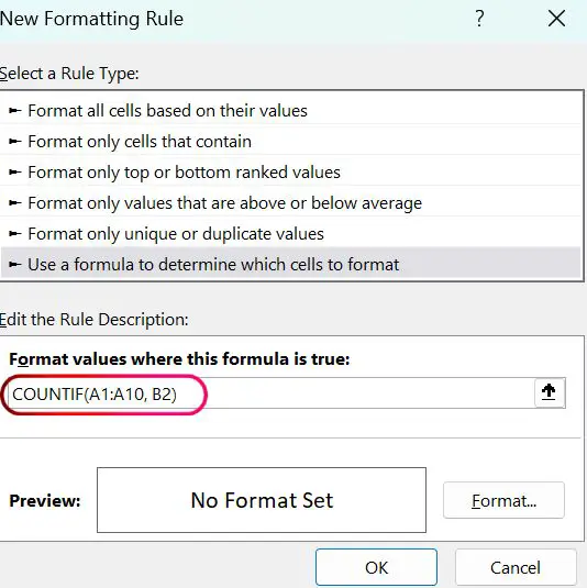
Step 2: Drag the formula down the column and it will count the number of times the specified value appears in the given range. If the count is greater than 1, then you have a duplicate.
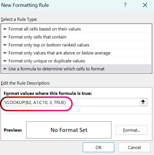
Step 3: VLOOKUP is a great way to identify duplicates when working with multiple columns of data. It allows you to retrieve the value of a specific cell in the table, based on the value of another cell.
The formula for VLOOKUP is “=VLOOKUP(lookup_value, table_array, col_index_num, [range_lookup]).
Replace the “lookup_value” with the value you want to look for, “table_array” with the range of cells containing the data you want to search, “col_index_num” with the column number containing the value you want to return, and “range_lookup” with either TRUE or FALSE, depending on if you want an exact or approximate match. For example, “=VLOOKUP(B2, A1:C10, 3, TRUE)”
Step 4: Drag the formula down the column, VLOOKUP will check the value against the table array, and if the value is found it will return the specified column value, and if not it will return “#N/A”.
Step 5: Now you can easily check which values have been returned as “#N/A” and see that as duplicates.
Both COUNTIF and VLOOKUP are powerful and versatile formulas that can be used to identify duplicates in Excel.
These formulas are more advanced then the previous ones and might require some practice and getting used to, but once you master them, you’ll be able to tackle any data analysis task like a pro!
Troubleshooting Common Issues when Identifying Duplicates in Excel
We’ve covered some great ways to identify duplicates in Excel, but as with anything, there can be some bumps in the road.
In this section, we’ll go over some common issues that can arise when identifying duplicates in Excel, and some tips for troubleshooting them.
First, one of the most common issues is when the “Remove Duplicates” feature or “Conditional Formatting” doesn’t seem to be working as expected.
Make sure that you’ve selected the correct range of cells and that you’ve included any headers or labels in your selection.
Also, make sure that your data is in the correct format, such as all being in the same date format, or text case format.
Another common issue is when the COUNTIF or VLOOKUP formula returns unexpected results.
Make sure that you’ve entered the correct range and value in the formula, and double-check that your column and row references are correct.
Another thing to keep in mind is that there may be “similar” duplicates which are not identical and may not be caught by these functions.
For example: “NY” and “New York” or “01/01/2022” and “January 1, 2022”, these kind of duplicates may require a different approach.
Finally, if you’re having trouble with any of these methods, don’t hesitate to consult the help resources provided by Microsoft or other online resources.
There are plenty of tutorials, videos, and forums that can help you with specific issues.
Keep in mind that identifying duplicates in Excel is an ongoing process, and you may need to repeat these steps periodically as your data changes or grows.
However, by following these tips and troubleshooting common issues, you’ll be able to organize your data and take your analysis to the next level!
Conclusion
In conclusion, identifying duplicates in Excel is an important step in keeping your data organized and accurate.
Excel offers several built-in tools, including the “Remove Duplicates” feature, “Conditional Formatting” and formulas like COUNTIF and VLOOKUP, to make the process easy and straightforward.
With this guide, you should be able to tackle any duplicate data in your spreadsheets and move on to your analysis with confidence.
It’s important to note that identifying duplicates is an ongoing process, you may need to repeat these steps periodically as your data changes or grows.
But with the methods and techniques provided in this post, you’ll be ready to handle any duplicate data that comes your way. Stay organized, stay accurate and happy analyzing!