
Hey there, Are you tired of staring at bland and unorganized tables in Google Sheets?
Well, have no fear, because today we’re diving into the world of table formatting and trust me, it’s going to be a game changer.
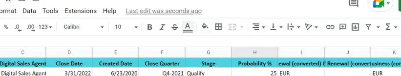
Whether you’re working on a business proposal, a budget spreadsheet, or a data analysis project, formatting your tables is key to making your data clear and easy to understand.
So, grab your coffee and get ready to learn some awesome tips and tricks for formatting tables in Google Sheets like a pro!
Creating a Table
Alright, let’s get started with the basics: creating a table in Google Sheets. Here’s a step-by-step guide to help you get started:
- Open Google Sheets and select the sheet where you want to create a table.
- Highlight the cells that you want to include in your table.
- Go to the “Format” menu and select “Table.”
- A pop-up window will appear, allowing you to customize the table’s design.
- Select the design that you like best and click “OK.”
And voila! You now have a beautiful and organized table in your Google Sheets document.
But don’t stop there, you can also add rows and columns to your table by right-clicking on the table and selecting “Insert row above” or “Insert column left.” This is a great way to add more data to your table and keep it organized.
Creating a table in Google Sheets is super easy and can make a huge difference in the way your data is presented. So, give it a try and see for yourself.
If you run into any trouble, feel free to reach out, and we’ll be happy to help. Happy formatting!
Formatting Table Text
Now that you’ve got your table set up, it’s time to add some pizzazz! One of the easiest ways to do this is by formatting the text within your table. Here are a few tips to help you get started:
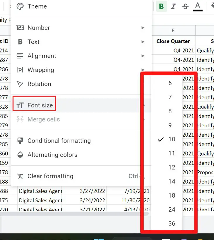
Font Size: To increase or decrease the font size of your text, simply highlight the cells you want to change, go to the “Format” menu, and select “Text size.” You can also use the shortcut “Ctrl + Shift + >” to increase the font size and “Ctrl + Shift + <” to decrease it.
Font Color: To change the font color of your text, highlight the cells you want to change, go to the “Format” menu, select “Text color” and pick your desired color.
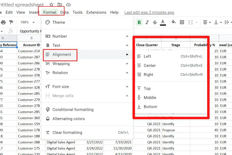
Alignment: To align your text within a cell, highlight the cells you want to change, go to the “Format” menu, and select “Align.” You can choose from left, center, or right alignment.
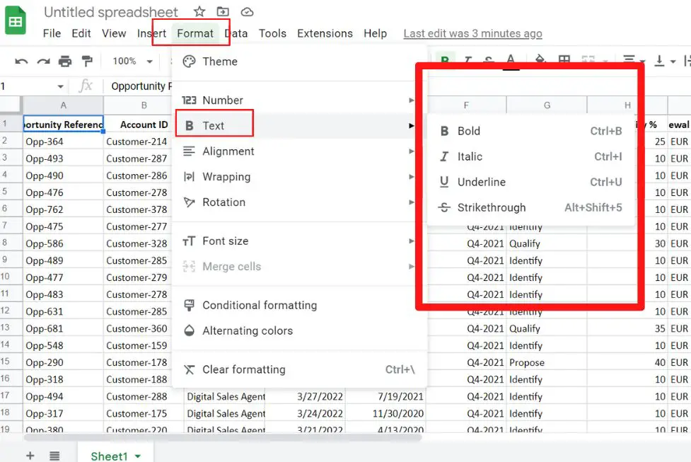
Bold, Italic, and Underline : You can use these options to highlight some specific cell text, you can find them on the toolbar above the sheet or you can use shortcut keys like ctrl+B for bold, ctrl+I for italic, and ctrl+U for underline.
These are just a few of the ways you can format the text within your table. Experiment with different options and find what works best for you.
Remember, the goal is to make your data clear and easy to understand, so don’t be afraid to play around with different formatting options. Happy formatting!
Formatting Table Borders
Now that we’ve covered text formatting, let’s move on to customizing the borders of your table. This is a great way to make your table stand out and add some visual interest to your data. Here are a few tips to help you get started:
- Border Color: To change the color of the borders in your table, highlight the cells you want to change, go to the “Format” menu, select “Borders” and pick your desired color.
- Border Weight: To change the weight (thickness) of the borders in your table, highlight the cells you want to change, go to the “Format” menu, select “Borders” and adjust the weight using the slider.
- Border Style: To change the style of the borders in your table, highlight the cells you want to change, go to the “Format” menu, select “Borders” and pick from the different style options like dotted, dashed, double, etc.
- Border all around : You can also select all the cells of the table and use the shortcut “Ctrl+Shift+&” to apply the border all around the cells.
- Clear all borders : If you want to remove all the borders of the table, you can use the shortcut “Ctrl+Shift+_”
As with text formatting, feel free to experiment with different border options to find what works best for your table.
Remember, the goal is to make your data stand out and be easy to understand, so don’t be afraid to play around with different formatting options. Happy formatting!
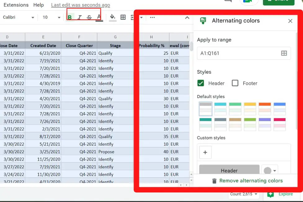
Formatting Table Background
So far, we’ve covered text formatting and border customization, but let’s not forget about the background of your table!
Changing the background color or adding a background image can add a whole new level of interest and personality to your data. Here are a few ways to get started:
- Background Color: To change the background color of your table, highlight the cells you want to change, go to the “Format” menu, select “Background color” and pick your desired color.
- Background Image: To add a background image to your table, highlight the cells you want to change, go to the “Format” menu, select “Background image” and upload the image you want to use. You can also use an image URL if the image is hosted on the web.
- Remove Background : To remove the background color or image of the table, you can use the shortcut “Ctrl+Shift+~”
These are just a few of the ways you can change the background of your table. Experiment with different options and find what works best for you.
Remember, the goal is to make your data stand out and be easy to understand, so don’t be afraid to play around with different formatting options. Happy formatting!
Merging and Splitting Cells
We’ve covered a lot of great ways to format your tables so far, but let’s not forget about the power of merging and splitting cells!
These tools can add an extra level of organization and flexibility to your data. Here’s a step-by-step guide to help you get started:
- Merging Cells: To merge cells within a table, simply select the cells you want to merge, right-click, and select “Merge cells.” You can also use the shortcut “Ctrl+Shift+1” to merge cells.
- Splitting Cells: To split cells within a table, first, select the cell you want to split, right-click, and select “Split cells.” A pop-up window will appear, allowing you to choose the number of columns and rows you want to split the cell into.
Merging and Splitting Cells is a powerful tool to customize the table cells to your needs. You can also use this feature to make a specific cell or row more prominent or to group some cells together.
Merging and splitting cells can be a great way to add an extra level of organization and flexibility to your data.
So don’t be afraid to experiment with different ways to use these tools to make your table even more polished and professional. Happy formatting!
Sorting and Filtering Data
We’re almost at the end of our journey, but we can’t forget about the importance of sorting and filtering data in your tables. These tools will make it easy to organize and analyze your data, so let’s dive in!
- Sorting Data: To sort data within a table, simply click on the column header you want to sort by, and Google Sheets will automatically sort the data in ascending order. To sort in descending order, simply click on the column header again.
- Filtering Data: To filter data within a table, click on the filter button located on the toolbar above the sheet. A drop-down menu will appear, allowing you to filter by specific values, conditions, or even create a custom filter.
- Advanced Filtering: You can also use advanced filtering options like filter by condition, filter by values, filter by selected cells and many more by going to the “Data” menu and selecting “Filter”
- You can also clear the filters by using the shortcut “Ctrl+Shift+L”
Sorting and filtering data can be a powerful way to quickly and easily organize and analyze your data. So don’t be afraid to play around with these tools and see how they can help you make sense of your data. Happy formatting!
Conclusion
Well, there you have it, We’ve covered a lot of great tips and tricks for formatting tables in Google Sheets, from text formatting and border customization to merging and splitting cells and sorting and filtering data.
To sum up, we’ve learned how to create a table in Google Sheets, format the text, customize the borders, change the background color or add a background image, merge and split cells, sort and filter data.
But the most important thing to remember is that formatting your tables is key to making your data clear and easy to understand. So, don’t be afraid to play around with different formatting options and see what works best for you.
And don’t forget, we’re always here to help if you have any questions or need some guidance. So don’t hesitate to reach out. We hope you’ve enjoyed this post and found it helpful. Happy formatting!